Chapter 3: Robot control

Last chapter we talked about how to model a robot: how its state evolves over time in response to control inputs. This chapter we ask the next natural question: how do we actually make the robot move the way we want?

More specifically, we want to choose control inputs $u$ that drive the robot toward a desired state, trajectory, or behaviour. In Chapter 2 we wrote models such as

$$x_{k+1} = f(x_k, u_k),$$

where $x_k$ is the robot state and $u_k$ is the control input. Control is about choosing $u_k$ so that the resulting sequence of states does something useful.

For example, we might want a robot to drive to a point, follow a path, stabilise around a desired pose, track a moving object, or move while respecting limits on velocity, acceleration, torque, clearance, or energy use.

Open-loop control

The simplest form of control is open-loop control. In open-loop control, we compute a sequence of control inputs ahead of time,

$$u_0, u_1, u_2, \dots,$$

and then execute them without checking what actually happened. There is no correction, no feedback, and no adaptation. We simply apply the planned commands and assume the robot follows them.

This can work when the system is predictable, the model is accurate, and disturbances are small. In that case, a planner can produce a trajectory and a corresponding sequence of actions, and the robot can execute that sequence directly.

The problem is that real robots rarely live in that world. Wheels slip, motors saturate, sensors are noisy, surfaces are uneven, loads change, models are approximate, and humans do unpredictable things. In open loop, small errors are not corrected. They accumulate over time, and eventually the robot may end up very far from where we intended.

Open-loop control is therefore useful as a starting point, but it is usually not enough for reliable robotics.

Feedback control loops

A more robust idea is to measure what actually happened and correct for it. This gives us a feedback loop.

Suppose we have a desired state, or reference, $x_d$, and an actual state $x$. The controller compares these quantities, computes an error, and chooses a control input $u$ based on that error. The robot then moves, we measure the new state, and the process repeats.

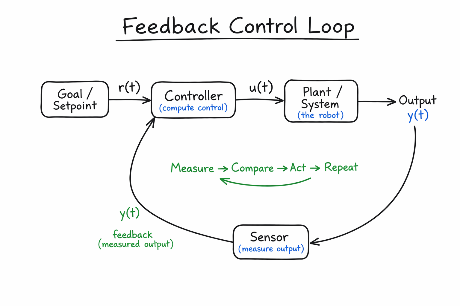
If $x_d$ is a fixed point, the problem is usually called regulation or setpoint control. If $x_d$ changes over time, the problem is usually called trajectory tracking. In both cases, the key idea is the same: use measurement to reduce error.

Feedback is one of the central ideas in robotics because it lets us handle uncertainty. We do not need the model to be perfect. We only need enough information to notice when we are wrong and correct the behaviour.

PID control

The most common starting point for feedback control is PID control, which stands for Proportional-Integral-Derivative control.

For a desired signal $x_d(t)$ and measured signal $x(t)$, define the error

$$e(t) = x_d(t) - x(t).$$

A continuous-time PID controller chooses the control input as

$$u(t) = K_p e(t) + K_i \int_0^t e(\tau)\,d\tau + K_d \frac{de(t)}{dt}.$$

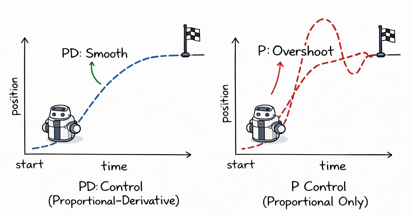
Each term plays a different role. The proportional term pushes the system toward the goal. A larger error produces a larger correction. The derivative term damps the response by reacting to how quickly the error is changing, which helps reduce overshoot and oscillation. The integral term accumulates past error, which helps remove steady-state error caused by bias, friction, gravity, model mismatch, or other persistent disturbances.

In discrete time, with time step $\Delta t$, a practical PID controller is often written as

$$e_k = x_{d,k} - x_k,$$ $$I_k = I_{k-1} + e_k \Delta t,$$ $$D_k = \frac{e_k - e_{k-1}}{\Delta t},$$

and

$$u_k = K_p e_k + K_i I_k + K_d D_k.$$

The gains $K_p$, $K_i$, and $K_d$ determine the behaviour of the controller. Increasing $K_p$ usually makes the system respond more strongly to error, but too much proportional gain can cause oscillation or instability. Increasing $K_d$ adds damping, but derivative control is sensitive to measurement noise. Increasing $K_i$ helps eliminate steady-state error, but too much integral action can cause slow oscillations or integral windup, where accumulated error becomes too large and the controller continues applying excessive control even after the system has moved close to the target. PD controller (no I term) is often more common in robotics because the I term can cause more practical trouble than benefit.

PID control is popular because it is simple, fast, interpretable, and often effective. It is widely used in low-level robot control, such as velocity control, joint control, heading control, altitude control, and temperature or motor regulation.

However, PID also has limitations. It does not explicitly know about the robot dynamics, does not automatically handle coupling between dimensions, does not optimise a cost function, and does not naturally enforce constraints such as actuator limits, collision avoidance, torque limits, or maximum curvature. PID is therefore useful, but not a complete solution for all robot control problems.

Example: driving to a goal

Consider a simple mobile robot with state

$$x = (x, y, \theta),$$

and control input

$$u = (v, \omega),$$

where $v$ is linear velocity and $\omega$ is angular velocity.

Suppose the goal position is $(x_g, y_g)$. The robot can compute the distance to the goal as

$$r_k = \sqrt{(x_g - x_k)^2 + (y_g - y_k)^2},$$

and the desired heading angle as

$$\theta_{g,k} = \operatorname{atan2}(y_g - y_k, x_g - x_k).$$

The heading error is then

$$e_{\theta,k} = \operatorname{wrap}(\theta_{g,k} - \theta_k),$$

where $\operatorname{wrap}(\cdot)$ maps the angle error into a range such as $[-\pi, \pi)$.

A simple proportional controller might choose

$$\omega_k = K_{p\theta} e_{\theta,k},$$

and

$$v_k = K_{pr} r_k.$$

This controller turns toward the goal and drives faster when the robot is farther away. In practice, we would usually also saturate the controls so that

$$|v_k| \leq v_{\max}, \qquad |\omega_k| \leq \omega_{\max}.$$

We might also reduce $v_k$ when the heading error is large, because driving forward quickly while facing away from the goal can produce poor behaviour.

This kind of controller is simple but surprisingly effective. It also illustrates a general theme in robotics: many useful controllers are built by combining geometric insight, feedback, and practical constraints.

LQR: Linear Quadratic Regulator

PID control is usually tuned directly in terms of gains. LQR takes a more formal approach. Instead of choosing gains by hand, we define a mathematical objective and derive the feedback controller that minimises it.

Assume the robot dynamics are linear and discrete time:

$$x_{k+1} = A x_k + B u_k.$$

Here, $x_k \in \mathbb{R}^n$ is the state, $u_k \in \mathbb{R}^m$ is the control input, $A$ describes how the state evolves without control, and $B$ describes how control inputs affect the state.

For regulation around a goal state $x_g$, define the state error

$$\tilde{x}_k = x_k - x_g.$$

If $x_g$ is an equilibrium state with corresponding equilibrium control $u_g$, we can similarly define

$$\tilde{u}_k = u_k - u_g.$$

The infinite-horizon discrete-time LQR problem is to choose a sequence of controls that minimises

$$J = \sum_{k=0}^{\infty} \left( \tilde{x}_k^T Q \tilde{x}_k + \tilde{u}_k^T R \tilde{u}_k \right),$$

subject to the linear dynamics.

The matrix $Q \succeq 0$ penalises state error, while $R \succ 0$ penalises control effort. Large values in $Q$ mean that errors in the corresponding state variables are expensive. Large values in $R$ mean that control effort is expensive. In this sense, LQR balances performance against effort.

The solution has a particularly important form:

$$\tilde{u}_k = -K \tilde{x}_k.$$

Equivalently,

$$u_k = u_g - K(x_k - x_g).$$

So LQR is still a feedback controller. The difference is that the feedback gain $K$ is not chosen by trial and error. It is computed from the system matrices $A$ and $B$ and the cost matrices $Q$ and $R$.

For the infinite-horizon discrete-time case (your robot and controller live forever), the gain is

$$K = (R + B^T P B)^{-1}B^T P A,$$

where $P$ is the positive semidefinite solution of the discrete algebraic Riccati equation

$$P = A^T P A - A^T P B(R + B^T P B)^{-1}B^T P A + Q.$$

This result is powerful because it gives an optimal stabilising controller for a linear system under a quadratic cost, assuming some controllability and stabilisability conditions are satisfied.

There is also a finite-horizon (your robot or its task lives for a finite time) version of LQR, where the cost is defined over $N$ time steps:

$$J = x_N^T Q_f x_N + \sum_{k=0}^{N-1} \left(x_k^T Q x_k + u_k^T R u_k\right).$$

In that case, the optimal gains vary with time and are computed by a backward Riccati recursion. This finite-horizon form is important because it connects directly to trajectory tracking, iLQR, and MPC.

LQR is elegant and useful, but it has limits. It assumes linear dynamics, quadratic costs, and usually does not include hard constraints directly. For nonlinear robots, we often linearise the dynamics around an operating point or nominal trajectory, then apply LQR locally.

Kalman, R. E. (1960). "Contributions to the Theory of Optimal Control." Boletin de la Sociedad Matematica Mexicana, 5(2), 102-119.

iLQR: iterative Linear Quadratic Regulator

LQR works beautifully for linear systems, but robots are often nonlinear. A mobile robot, for example, may have dynamics such as

$$x_{k+1} = f(x_k, u_k),$$

where $f$ contains terms like $\sin\theta$, $\cos\theta$, contacts, saturations, or other nonlinear effects.

The main idea of iterative LQR, or iLQR, is to repeatedly approximate a nonlinear optimal control problem by a local linear-quadratic problem.

Suppose we want to minimise a finite-horizon cost

$$J = \ell_f(x_N) + \sum_{k=0}^{N-1} \ell(x_k, u_k),$$

subject to

$$x_{k+1} = f(x_k, u_k).$$

Starting from an initial guess for the control sequence, iLQR first simulates the system forward to obtain a nominal trajectory

$$\bar{x}_0, \bar{x}_1, \dots, \bar{x}_N, \qquad \bar{u}_0, \bar{u}_1, \dots, \bar{u}_{N-1}.$$

It then linearises the dynamics around that trajectory:

$$\delta x_{k+1} \approx A_k \delta x_k + B_k \delta u_k,$$

where

$$A_k = \left.\frac{\partial f}{\partial x}\right|_{\bar{x}_k,\bar{u}_k}, \qquad B_k = \left.\frac{\partial f}{\partial u}\right|_{\bar{x}_k,\bar{u}_k}.$$

The cost is also approximated locally by a quadratic expansion. This produces a local LQR-like problem, which can be solved efficiently using a backward pass. The backward pass computes both a feedforward correction and a feedback gain, giving a local control update of the form

$$\delta u_k = k_k + K_k \delta x_k.$$

The algorithm then performs a forward rollout with updated controls, checks whether the cost improved, and repeats the process until convergence.

At a high level, iLQR alternates between two steps. The forward pass simulates the nonlinear system using the current controls. The backward pass solves a local linear-quadratic approximation to improve those controls.

This makes iLQR much more suitable than LQR for nonlinear robot motion problems. It is often used for trajectory optimisation, legged locomotion, manipulation, and dynamic motion planning.

However, iLQR is still a local method. Its solution depends on the initial guess, and because the original nonlinear problem may be non-convex, the algorithm can converge to a local minimum. It also does not naturally handle hard constraints unless modified. Related methods such as DDP, constrained iLQR, and sequential quadratic programming address some of these issues.

In practice, iLQR is often used to compute a good nominal trajectory, and a feedback controller is then used to track that trajectory on the real robot.

Li, W. and Todorov, E. (2004). "Iterative Linear Quadratic Regulator Design for Nonlinear Biological Movement Systems." In Proceedings of the 1st International Conference on Informatics in Control, Automation and Robotics (ICINCO), pp. 222-229.

MPC: Model Predictive Control

Model Predictive Control, or MPC, takes another step toward practical robot control. Instead of solving an optimal control problem once and committing to the whole solution, MPC repeatedly solves a finite-horizon control problem as the robot moves.

At time step $k$, MPC uses the current state estimate $x_k$ as the initial condition and solves an optimisation problem over a prediction horizon of length $N$:

$$\min_{u_{k|k}, \dots, u_{k+N-1|k}} \ell_f(x_{k+N|k}) + \sum_{i=0}^{N-1} \ell(x_{k+i|k}, u_{k+i|k}),$$

subject to the model dynamics

$$x_{k+i+1|k} = f(x_{k+i|k}, u_{k+i|k}),$$

and, when needed, constraints such as

$$x_{k+i|k} \in \mathcal{X}, \qquad u_{k+i|k} \in \mathcal{U}.$$

Here, $x_{k+i|k}$ means the state predicted for time $k+i$ using information available at time $k$. The sets $\mathcal{X}$ and $\mathcal{U}$ describe allowable states and controls. These might represent actuator limits, velocity limits, collision constraints, workspace boundaries, torque limits, or safety margins.

After solving this optimisation problem, MPC applies only the first control input,

$$u_k = u_{k|k}^*,$$

then observes the new state, shifts the horizon forward, and solves again.

This repeated re-planning is the defining feature of MPC. It gives MPC some important advantages. It can respond to disturbances, update its plan as new sensor information arrives, and handle constraints explicitly. This makes it especially useful in robotics, autonomous driving, process control, aerial robotics, legged robots, and manipulation.

The trade-off is computation. MPC requires solving an optimisation problem online, often at every control step. The difficulty of that optimisation problem depends on the model, the cost, the constraints, and the horizon length.

For linear dynamics with quadratic costs and linear constraints, MPC becomes a quadratic program, which can often be solved reliably and quickly. For nonlinear dynamics, nonlinear MPC is more general but more computationally demanding, and it may require careful initialisation and solver tuning.

MPC can be viewed as combining planning and feedback. Like planning, it predicts future behaviour using a model. Like feedback control, it repeatedly updates the plan based on the measured state.

Mayne, D. Q., Rawlings, J. B., Rao, C. V., and Scokaert, P. O. M. (2000). "Constrained model predictive control: Stability and optimality." Automatica, 36(6), 789-814.

Comparing PID, LQR, iLQR, and MPC

PID is often the simplest useful controller. It is easy to implement, computationally cheap, and works well for many low-level control tasks. Its main weakness is that it does not explicitly use a model of the full system dynamics or optimise a global objective.

LQR uses a linear model and a quadratic cost to compute an optimal feedback gain. It is more systematic than PID and gives strong theoretical guarantees for suitable linear systems, but it is limited by its assumptions about linearity and unconstrained control.

iLQR extends the LQR idea to nonlinear systems by repeatedly linearising the dynamics and quadratically approximating the cost around a nominal trajectory. It is powerful for trajectory optimisation, but it is local and can be sensitive to the initial guess.

MPC repeatedly solves a finite-horizon optimal control problem online. It is powerful because it can incorporate constraints and adapt to new information, but it is usually more computationally expensive than PID or LQR.

These methods are not mutually exclusive. A robot might use a planner to generate a route, iLQR or MPC to produce a dynamically feasible trajectory, and PID loops at the motor level to track commanded velocities or torques.

Key Papers

Kalman, R. E. (1960). "Contributions to the Theory of Optimal Control." Boletin de la Sociedad Matematica Mexicana, 5(2), 102-119.

Li, W. and Todorov, E. (2004). "Iterative Linear Quadratic Regulator Design for Nonlinear Biological Movement Systems." In Proceedings of ICINCO, pp. 222-229.

Mayne, D. Q., Rawlings, J. B., Rao, C. V., and Scokaert, P. O. M. (2000). "Constrained model predictive control: Stability and optimality." Automatica, 36(6), 789-814.

Coming up next

So far, we have assumed that we can measure the state of the robot accurately enough to use it for feedback. Next, we look at what happens when we cannot directly observe the state and must estimate it from noisy, delayed, and incomplete sensor measurements.

→ Chapter 4: State Estimation