Chapter 4: Localisation and state estimation

Uncertainty and beliefs

So far, we have spoken about how to represent our robot and our world and model the dynamics of how things change when we interact with it, but we haven't discussed how we obtain this information. In practice we can never know the ground truth state of our robot and the world, and always measure or sense it subject to some error. There may also be completely un-modelled aspects on stochastic effects in the world, which also introduce uncertainty. We need methods to cope with this uncertainty - and the best language to think about uncertainty is probability.

Typically, we are taught to reason about probabilities in terms of frequencies - if I roll a dice 10 times, what are the chances I roll a 6? This frequentist perspective doesn't really match the robotics problem we face, so instead we tend to think about probability as a belief: given what I have sensed in the world, I believe my state is x with some probability.

In robotics, we can rarely trust our sensors. Instead, we may think about the likelihood of making some observation $z_t$, $p(z_t|x_t)$ in a given state. As an example, think about a temperature sensor that measures temperature with zero-mean gaussian noise of standard deviation 5 degrees. If the true temperature were 25 degrees, and our sensor measured 25.05 degrees, the likelihood of making this observation would be $\mathcal{N}(z_t|x_t,\sigma) = \mathcal{N}(25.05|25,5)$, quite probable. Here $\mathcal{N}$ is shortand for a Gaussian distribution over $z_t$ with mean $x_t$ and standard deviation $\sigma$. However, if the true temperature were 0 degrees, it is much less likely our temperature sensor would return a measurement of 25.05 degrees.

But we may have other sources of information. What if for example we knew that our temperature sensor is located in Antartica? When we incorporate this $prior$, that 0 degree temperature starts to seem a lot more probable.

Bayes Rule

Bayes rule is a law of probability (you can easily derive this using conditional probability laws) that gives us a principled way of combining prior information with likelihoods. We write

$$p(x_t|z_t) = \frac{p(z_t|x_t)p(x_t)}{p(z_t)}$$

Our posterior belief, the probability that I am in state $x_t$, given the observation $z_t$ is equal to the likelihood of seeing observation $z_t$ if I were in state $x_t$, multipled by the prior belief that I was in state $x_t$, normalised by the marginal likelihood of ever seeing the observation $z_t$.

We call

$$p(z_t) = \int p(z_t|x_t) p(x_t) d x_t$$

a marginal likelihood because it marginalises out all the possible ways we could get an observation $z_t$, by averaging (takes an expectation) over all the states $x_t$ in proportion to the probabability of these occuring.

Recursive state estimation

Bayes rule gave us a way of expressing our belief that our robot was in a state given a single observation, but in practice we are interested in the conditional probability distibution: $p(x_t|z_{1:t})$ - given all observations or measurements $z$ taken at times steps $1$ to $t$, what is the probability that my robot (or world) is in the state $x_t$. We refer to this as a state estimation or tracking problem.

Using Bayes rule, we can express this as

$$p(x_t|z_{1:t}) = \frac{p(z_{1:t}|x_t) p(x_t)}{p(z_{1:t})} = \frac{p(z_{t}|x_t,z_{1:t-1}) p(z_{1:t-1}|x_t)|p(x_t)}{p(z_t|z_{1:t-1})p(z_{1:t-1})} \quad \text {factorising and conditioning the joint distribution}$$ $$p(x_t|z_{1:t}) = \frac{p(z_{t}|x_t) p(x_t|z_{1:t-1})}{p(z_t|z_{1:t-1})} \quad \text{Simplifiying the likelihood and applying another Bayes rule}$$

Which can in turn be broken down into two steps:

$$p(x_t|z_{1:t-1}) = \int p(x_t|x_{t-1}) p(x_{t-1}|z_{1:t-1}) d x_{t-1} \quad \text{Predict}$$ $$p(x_t|z_{1:t}) = \frac{p(z_{t}|x_t) p(x_t|z_{1:t-1})}{p(z_t|z_{1:t-1})} \quad \text{Update}$$

The recursion above is very powerful, it provides a sequential way of updating our belief in a robot state as new information comes in. Looking at the equations above, we can see what we need to make this happen. We start with a prior belief in our robot state $p(x_0)$.

We then use a dynamics model to predict where our robot may be. Last chapter, when we introduced robot models we saw that these could be expressed as $x_t = f(x_{t-1},u_{t},\epsilon)$, with $\epsilon$ our uncertainty or disturbances affecting our model. Another way to describe this is that our dynamics are a probabalistic transtion $p(x_t|x_{t-1},u_{t-1})$, given a state and action at time $t-1$, what is the probability that my robot is in the state $x_t$. For simplicity, we will drop the $u$ for now. The equations above use this to make a prediction about where our robot could be after taking some action.

We then get a measurement or observation as multiply the likelihood of obtaining this in a given state by the predicted probability of being in that state to get a posterior belief. This becomes the prior for the next recursion. As we repeat this, we accumulate information and refine our beliefs over time.

Let's make this more concrete with an example. My robot starts somewhere near the position (0,0). We use the dynamics to make a prediction about all the places it could possibily end up for a given movement command. We then make a measurement, and reweight this by the chances of getting that measurement for each of these places. We now use this as the new belief for our robot state, and repeat.

This is a general rule that applies regardless of dynamics, sensors or representations - neuroscientists often talk about Bayesian brains. Lets look at some common assumptions, representations and models.

Discrete Bayes (Histogram) filters

The recursive state estimation equations above are completely general, but in many cases they are hard to compute exactly. One simple way to make them tractable is to assume that the state can only take one of a finite number of values. Instead of representing our belief as a continuous probability density, we represent it as a set of probabilities over bins or cells. This is why these are often called histogram filters.

Suppose our state $x_t$ can take values from a finite set $\{x^1, x^2, \dots, x^N\}$. Our belief is then just a categorical distribution:

$$\mathrm{bel}_t(i) = p(x_t = x^i \mid z_{1:t})$$

where $\mathrm{bel}_t(i)$ is the probability that the robot is in state $x^i$ at time $t$.

The prediction step becomes a sum rather than an integral:

$$\overline{\mathrm{bel}}_t(i) = p(x_t = x^i \mid z_{1:t-1}) = \sum_{j=1}^N p(x_t = x^i \mid x_{t-1} = x^j)\,\mathrm{bel}_{t-1}(j)$$

This says that the probability of being in bin $i$ at time $t$ is found by considering all the ways we could have arrived there from every bin $j$ at time $t-1$, weighted by how likely it was that we were in bin $j$.

The update step is then

$$\mathrm{bel}_t(i) = \eta \, p(z_t \mid x_t = x^i)\,\overline{\mathrm{bel}}_t(i)$$

where $\eta$ is a normalising constant chosen so that the probabilities sum to one:

$$\eta = \frac{1}{\sum_{i=1}^N p(z_t \mid x_t = x^i)\,\overline{\mathrm{bel}}_t(i)}$$

So the full discrete Bayes filter is

$$\overline{\mathrm{bel}}_t(i) = \sum_{j=1}^N p(x_t = x^i \mid x_{t-1} = x^j)\,\mathrm{bel}_{t-1}(j)$$ $$\mathrm{bel}_t(i) = \eta \, p(z_t \mid x_t = x^i)\,\overline{\mathrm{bel}}_t(i)$$

This is perhaps the most direct implementation of recursive state estimation. It works for arbitrary probability distributions and can represent multiple hypotheses very naturally. For example, if a robot in a corridor cannot distinguish between two similar-looking locations, the histogram filter can represent a belief with two distinct peaks.

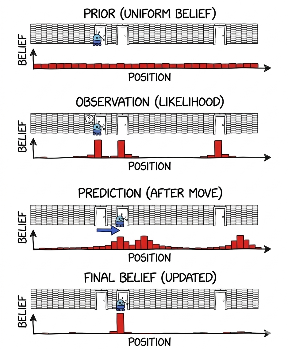
This famous example is taken from the paper

Fox, Dieter, Wolfram Burgard, and Sebastian Thrun. "Markov localization for mobile robots in dynamic environments." Journal of artificial intelligence research 11 (1999): 391-427.

The downside is that the number of bins grows very quickly with state dimension, but you can probably already see how this can be used with the occupancy grid map representation we saw in Chapter 1. For a one or two-dimensional state this may be fine, but for higher-dimensional states it quickly becomes computationally expensive.

---

Kalman filters

A different approach is to assume that the uncertainty in our state can be represented by a Gaussian distribution. Instead of tracking the full probability distribution, we only track its mean and covariance. This gives a very compact representation, and under linear-Gaussian assumptions the recursion can be computed exactly.

Suppose our dynamics are linear:

$$x_t = A x_{t-1} + B u_t + \epsilon_t$$

with process noise

$$\epsilon_t \sim \mathcal{N}(0,Q)$$

and our measurement model is also linear:

$$z_t = C x_t + \delta_t$$

with measurement noise

$$\delta_t \sim \mathcal{N}(0,R)$$

If our prior at time $t-1$ is Gaussian,

$$p(x_{t-1}\mid z_{1:t-1}) = \mathcal{N}(x_{t-1}; \mu_{t-1}, \Sigma_{t-1})$$

then the predicted state is also Gaussian:

$$p(x_t \mid z_{1:t-1}) = \mathcal{N}(x_t; \overline{\mu}_t, \overline{\Sigma}_t)$$

with

$$\overline{\mu}_t = A\mu_{t-1} + B u_t$$ $$\overline{\Sigma}_t = A \Sigma_{t-1} A^\top + Q$$

These are the prediction equations. The mean is propagated through the dynamics, while the covariance grows due to both prior uncertainty and process noise.

Once we receive a measurement $z_t$, we update our belief. The innovation (or residual) is:

$$y_t = z_t - C \overline{\mu}_t$$

The innovation covariance is:

$$S_t = C \overline{\Sigma}_t C^\top + R$$

The Kalman gain is:

$$K_t = \overline{\Sigma}_t C^\top S_t^{-1}$$

The posterior mean and covariance are then:

$$\mu_t = \overline{\mu}_t + K_t y_t$$ $$\Sigma_t = (I - K_t C)\overline{\Sigma}_t$$

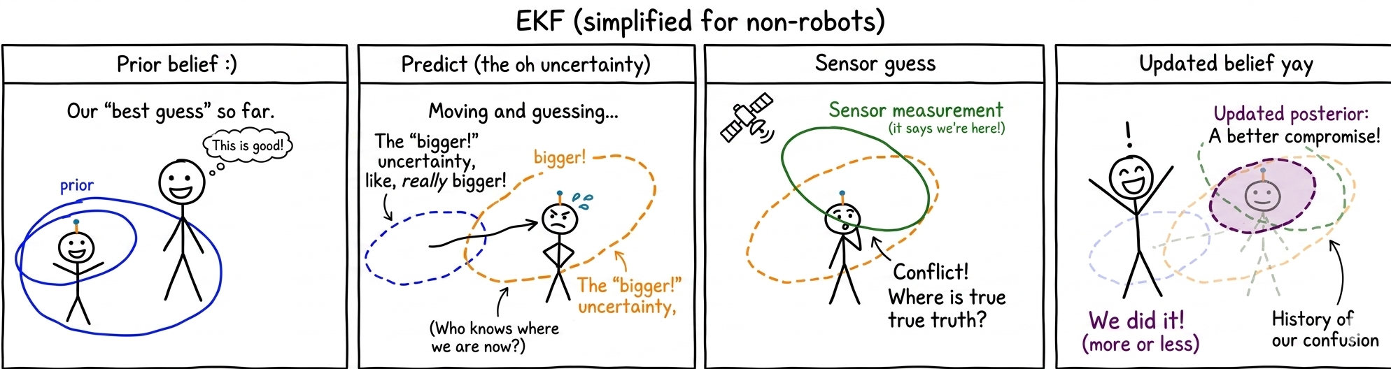
The Kalman filter is optimal for linear systems with Gaussian noise. This provides a balance between trusting the model and trusting the measurements, depending on their respective uncertainties.

Kalman, R. E. (1960). "A New Approach to Linear Filtering and Prediction Problems." Journal of Basic Engineering, 82(1), 35–45.

There is a catch though, the Kalman filter can't handle multi-modal beliefs like the corridor example above. A Gaussian distribution only has one mode or peak.

Extended Kalman filters

Real robotic systems are rarely linear. The Extended Kalman Filter (EKF) adapts the Kalman filter to nonlinear systems by linearising the dynamics and measurement models around the current estimate.

Suppose our system is:

$$x_t = f(x_{t-1},u_t) + \epsilon_t, \qquad \epsilon_t \sim \mathcal{N}(0,Q)$$ $$z_t = h(x_t) + \delta_t, \qquad \delta_t \sim \mathcal{N}(0,R)$$

Predict

We propagate the mean through the nonlinear dynamics:

$$\overline{\mu}_t = f(\mu_{t-1},u_t)$$

We compute the Jacobian of the dynamics:

$$F_t = \left.\frac{\partial f}{\partial x}\right|_{x=\mu_{t-1},u=u_t}$$

and approximate the covariance:

$$\overline{\Sigma}_t = F_t \Sigma_{t-1} F_t^\top + Q$$

Update

We predict the measurement:

$$\hat{z}_t = h(\overline{\mu}_t)$$

Compute the Jacobian of the measurement model:

$$H_t = \left.\frac{\partial h}{\partial x}\right|_{x=\overline{\mu}_t}$$

Innovation:

$$y_t = z_t - \hat{z}_t$$

Innovation covariance:

$$S_t = H_t \overline{\Sigma}_t H_t^\top + R$$

Kalman gain:

$$K_t = \overline{\Sigma}_t H_t^\top S_t^{-1}$$

Posterior:

$$\mu_t = \overline{\mu}_t + K_t y_t$$ $$\Sigma_t = (I - K_t H_t)\overline{\Sigma}_t$$

The EKF works well when nonlinearities are mild, but it is only an approximation and can struggle when the system is highly nonlinear. Let's look at this for a wheeled mobile robot.

Julier, S. J. and Uhlmann, J. K. (1997). "A New Extension of the Kalman Filter to Nonlinear Systems." In Proceedings of SPIE, vol. 3068, pp. 182–193.

---

Particle filters

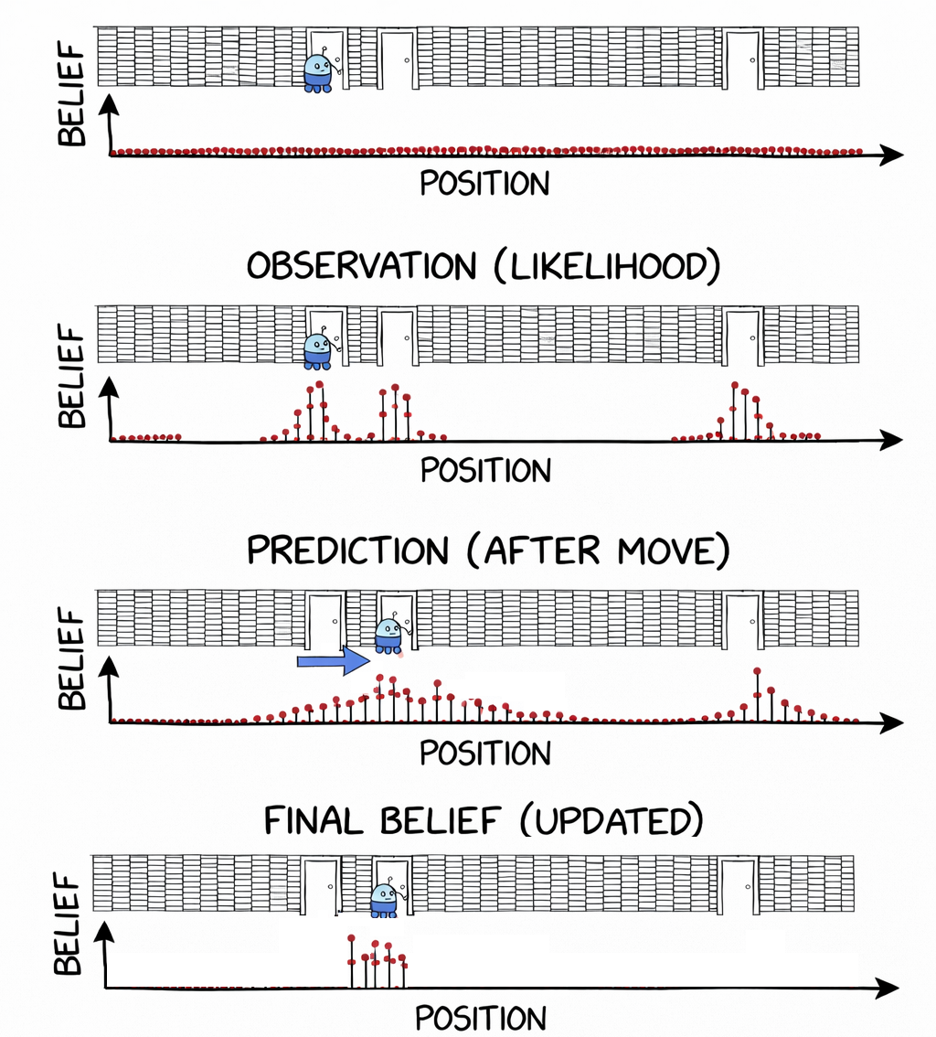
A third approach is to represent the belief distribution using a set of $M$ weighted samples or particles. This allows us to approximate arbitrary probability distributions, including multimodal ones while addressing some of the downsides of discretising the whole state space into a histogram.

We approximate the posterior as:

$$p(x_t \mid z_{1:t}) \approx \sum_{i=1}^M w_t^{(i)} \,\delta(x_t - x_t^{(i)})$$

where each particle $x_t^{(i)}$ is a hypothesis of the state, and $w_t^{(i)}$ is its weight.

At time $t-1$, we have:

$$\{x_{t-1}^{(i)}, w_{t-1}^{(i)}\}_{i=1}^M$$

Predict

We sample each particle forward:

$$x_t^{(i)} \sim p(x_t \mid x_{t-1}^{(i)}, u_t)$$

Update

We update weights using the likelihood:

$$\tilde{w}_t^{(i)} = w_{t-1}^{(i)} \, p(z_t \mid x_t^{(i)})$$

Normalise

$$w_t^{(i)} = \frac{\tilde{w}_t^{(i)}}{\sum_{j=1}^M \tilde{w}_t^{(j)}}$$

Resample

Resample particles according to $w_t^{(i)}$, then reset:

$$w_t^{(i)} = \frac{1}{M}$$

Particle filters are very flexible and can represent complex, multimodal beliefs. However, they can be computationally expensive, especially in high-dimensional state spaces. Another name for a particle filter is sequential Monte Carlo inference.

Gordon, N. J., Salmond, D. J., and Smith, A. F. M. (1993). "Novel approach to nonlinear/non-Gaussian Bayesian state estimation." IEE Proceedings F – Radar and Signal Processing, 140(2), 107–113.

Summary

All of these filters implement the same recursive Bayes estimation framework. The key difference lies in how the belief distribution is represented.

• Histogram filters use a discrete representation over bins.
• Kalman filters assume linear-Gaussian systems and track mean and covariance.
• Extended Kalman filters handle nonlinear systems via linearisation.
• Particle filters approximate the distribution using weighted samples.

Each method trades off accuracy, flexibility, and computational cost, and the right choice depends on the characteristics of the system being modelled. The estimation approach and abstraction also affects what we can control or how we plan so is an important design choice in any robotic application.

Sensor fusion

Sensor fusion is the general problem of combining information from multiple sensors to support robot state estimation. Importantly, this is not a separate problem from state estimation, it is the same recursive Bayes estimation framework with multiple sensor streams. We still make a prediction using the motion model and then perform correction using measurements; we simply repeat or combine updates from different sensors under the same posterior belief.

In other words, we are still estimating distributions like $p(x_t \mid z_{1:t})$, but now $z_t$ may include measurements from wheel odometry, IMU, camera, lidar, GNSS and other sources with different rates and noise characteristics.

You want an estimate of some state (often pose + velocity):

$$x_t = [\mathbf{p}_t,\;\mathbf{v}_t,\;\boldsymbol{\theta}_t,\;\mathbf{b}_t]$$

where $\mathbf{b}_t$ includes sensor biases (IMU bias, gyro drift, etc.).

Nearly all practical fusion fits the pattern:

• prediction using a motion model (often IMU integration)
• correction using measurements (camera/lidar/GPS/wheels)

Practical tuning heuristics

• If you trust a sensor too much, it will dominate and break you when it fails.
• If you trust it too little, you drift forever.

When in doubt:

• start conservative (higher measurement noise),
• then gradually tighten.

What to plot when debugging estimation

Plot over time:

• uncertainty/ innovation / residual norms (measurement minus prediction)
• estimated biases ($b_t$)
• velocity and yaw rate consistency
• pose drift vs ground truth (if available)
• number of inliers / matched features / scan match score

---

Key Papers

Kalman, R. E. (1960). "A New Approach to Linear Filtering and Prediction Problems." Journal of Basic Engineering, 82(1), 35–45.

Julier, S. J. and Uhlmann, J. K. (1997). "A New Extension of the Kalman Filter to Nonlinear Systems." In Proceedings of SPIE, vol. 3068, pp. 182–193.

Gordon, N. J., Salmond, D. J., and Smith, A. F. M. (1993). "Novel approach to nonlinear/non-Gaussian Bayesian state estimation." IEE Proceedings F, 140(2), 107–113.

Fox, D., Burgard, W., and Thrun, S. (1999). "Markov localization for mobile robots in dynamic environments." Journal of Artificial Intelligence Research, 11, 391–427.

Thrun, S., Burgard, W., and Fox, D. (2005). Probabilistic Robotics. MIT Press.

---

Coming up next

We can now estimate where our robot is. Next, we use this to navigate.

→ Chapter 5: Navigation